Colour alternating rows in an Excel worksheet – Option 1

In a large spreadsheet that has many columns of data it can be difficult following a specific row as you scroll to the right.  This is especially true if you have zoomed out so more data fits on the screen and the rows are smaller than usual.

Wouldn’t it be great if alternating rows in the workbook were coloured so you could more easily run your eye along a row?  You can do this with conditional formatting.

Select the rows you want coloured then:

1. On the Home tab in the Styles group, click on the Conditional Formatting button
2. Select New Rule…
3. In the New Formatting Rule dialog box, select the last option in the list: Use a formula to determine which cells to format
4. Add the following formula to the Format values where this formula is true text box: =MOD(ROW(),2)=1
   
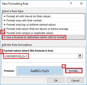
5. Click on the Format button and select a colour from the Fill tab
6. Click on OK twice

Notes:

• You can paste the formula in step 4 above, including the =,  into the text box, if you’d like
• In case you are wondering, the ROW function returns the row number and the Mod function divides it by 2.  In the formula above, odd rows will be coloured.  Change the 1 to a 0 and your workbook would look the same but even rows would be coloured.